
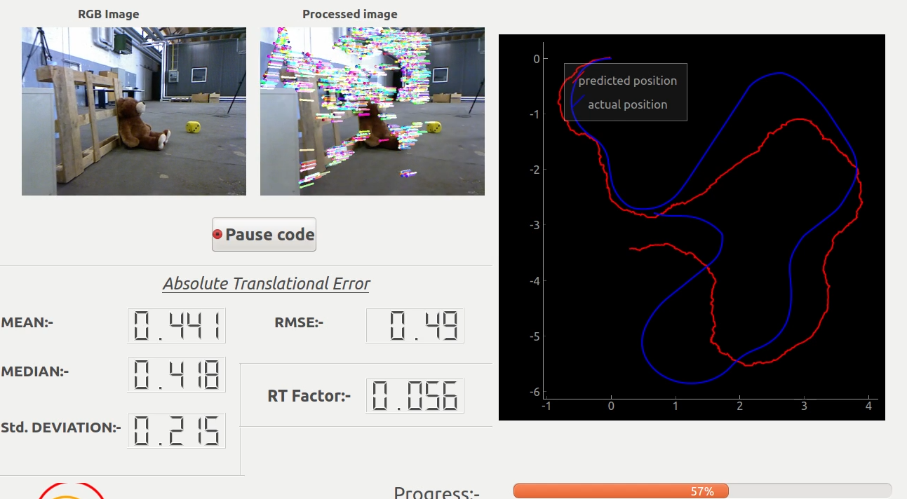
Using the Evaluator Software about which I have described here , I attempted my first Monocular Visual Odometry algorithm. Before proceeding further let’s look at the result (watch in fullscreen) .
If you observe the result closely you will notice that during the initial part of the path the predicted path more or less closely follows the actual path but during the latter part of the path the predicted path deviates largely from the actual path. This is due to the fact that the error in predicting the position during each step gets cumulated in the consecutive steps resulting in increasing deviation from the groundtruth as the algorithm proceeds.
This shortcoming of this algorithm can be avoided by implementing one or multiple of these methods:
-
Kalman Filter (if approximate process model can be formulated).
-
Bundle Adjustment.
-
Pose-graph optimization.
-
Loop closure detection.
Anyways I will be explaining my approach to the Monocular Visual Odometry algorithm. A details treatement about the basics of Visual Odometry is available at Dr.Scaramuzza’s site and here.
- Here is a brief outline of the steps involved in the Monocular Visual Odometry:-
1) Detect features from the first available image using FAST algorithm.
fast = cv2.FastFeatureDetector_create()
fast.setThreshold(fast_threshold) # set the threshold parameter
keypoints_prev = fast.detect(color_img,None)
2) Track the detected features in the next available image using Lucas-Kanade Optical Flow Algorithm.
img_new_gray = cv2.cvtColor(img_new_color , cv2.COLOR_BGR2GRAY) # first grayscale the image
lk_params = dict( winSize  = (50,50),
              maxLevel = 30,
              criteria = (cv2.TERM_CRITERIA_EPS | cv2.TERM_CRITERIA_COUNT, 10, 0.03)) # mention the Optical Flow Algorithm parameters
keypoints_new, st, err = cv2.calcOpticalFlowPyrLK(img_prev_gray, img_new_gray, keypoints_prev, None, **lk_params)
3) If the number of tracked features falls below a certain threshold:
if len(keypoints_new) < certain_no_of threshold:
 Detect features again in the previous image.

 Track those features in the next image.

 Else:

 Continue tracking the detected features in the next images.
4) Compute Essential Matrix from the corresponding points in two images using Nister’s 5 Point Algorithm.
essential_mat, = cv2.findEssentialMat(keypoints_prev , keypoints_new ,focal = fx , pp = (cx , cy), method = cv2.RANSAC ,prob=0.999, threshold=1.0) # replace with proper focal length and optical center of the camera
5) Recover relative camera rotation and translation from an estimated essential matrix and the corresponding points in two images, using cheirality check.
_,R ,t , = cv2.recoverPose(essential_mat , keypoints_prev , keypoints_new, focal = fx , pp = (cx , cy)) # replace with proper focal length and optical center of the camera
6) Triangulate the feature points from two consecutive images with the camera intrinsic matrix, rotation matrix and translation vector to reconstruct it to a 3D pointcloud.
K = np.array([[fx,0,cx],[0,fy,cy],[0,0,1]]) # set the intrinsic camera matrix
# The canonical matrix (set as the origin)
P0 = np.array([[1, 0, 0, 0],
               [0, 1, 0, 0],
               [0, 0, 1, 0]])
P0 = K.dot(P0)
# Rotated and translated using P0 as the reference point
P1 = np.hstack((R, t))
P1 = K.dot(P1)
cloud_new = cv2.triangulatePoints(P0, P1, point1, point2).reshape(-1, 4)[:, :3] # Triangulate the keypoints to a pointcloud and reshape it to a Nx3 shaped pointcloud.
7) Compute the relative scale -> The proper scale can then be determined from the distance ratio r between a point pair in pointcloud $X_{k-1}$ and a pair in pointcloud $X_k$ .
\[r = \frac{ \lvert \lvert X_{k-1,i} - X_{k-1,j} \rvert \rvert}{ \lvert \lvert X_{k,i} - X_{k,j} \rvert \rvert}\]For robustness, the scale ratios for many point pairs are computed and the mean (or in presence of outliers, the median) is used.
8) Concatenate the Rotation and Translational matrix along with the relative scale to obtain the predicted path.
\[R_{robot} = RR_{robot}\] \[t_{robot} = t_{robot} + scale * tR_{robot}\]Additional Heuristics:
Since the motion of the mobile robot in question does not have any sharp turn , we will will drop the predicted Rotation and translation if the rotation angle is more than 5 degrees in a single step.Also if the predicted translation vector moves in backward direction we will drop that prediction.
Global scale: If you plot the result of this above explained algorithm you will notice that the predicted path is off by a constant scale factor from the groundtruth. This is a common problem in Monocular Visual odometry as it has no intrinsic way to determine or predict the global scale . So the global scale factor has to be extracted from external information.
IMU odoemtry:
For IMU odometry I have implemented dead reckoning for predicting the robot path . But again this method is subject to cumulative errors. So IMU sensors solely are not used for poition estimation.
\[V_{avg_x} = \frac{(A_{x,t-1} + A_{x,t})}{2} * dt\] \[V_{avg_y} = \frac{(A_{y,t-1} + A_{y,t})}{2} * dt\] \[dx = V_{avg_x} * dt\] \[dy = V_{avg_y} * dt\]So here is the result:
In my next blog post I will try to produce better result by fusing the visual estimate and IMU estimate using Kalman filter.