In my previous blog post I have explained the basic steps involved in a Monocular Visual Odmetry algorithm. But the major drawback in the Monocular visual odometry is that prior global scale information has to be provided .

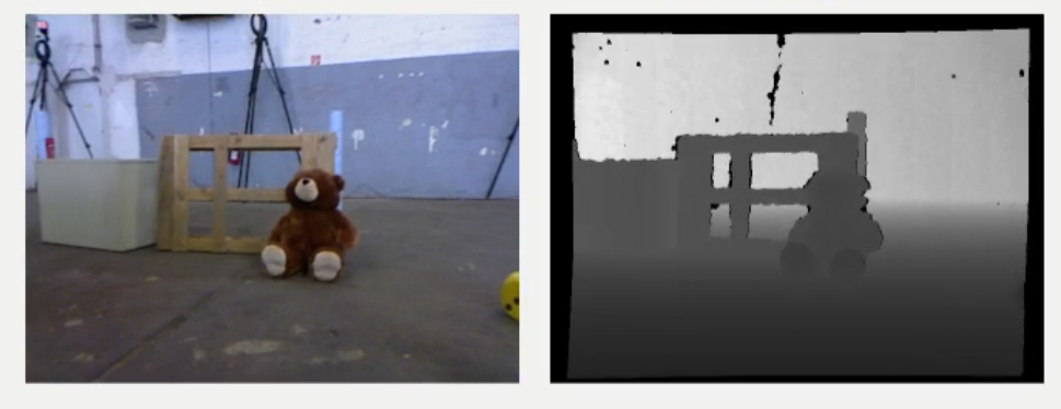
So if Depth image is available to the user along with the RGB image then the global scale information can be obtained from the depth image. I will explain the basic pipeline involved in pose prediction using RGBD odometry algorithm based on this paper¹. (Remember the color and depth image should be pre-registered.)

For testing the performance , accuracy and visualising the odometry algorithm I have used this software.

1) Detect features from the first available RGB image using FAST algorithm.

fast = cv2.FastFeatsureDetector_create()
fast.setThreshold(fast_threshold) # set the threshold parameter
keypoints_prev = fast.detect(color_img,None)

2) Track the detected features in the next available RGB image using Lucas-Kanade Optical Flow Algorithm.

img_new_gray = cv2.cvtColor(img_new_color , cv2.COLOR_BGR2GRAY) # first grayscale the image
lk_params = dict( winSize  = (50,50),
              maxLevel = 30,
              criteria = (cv2.TERM_CRITERIA_EPS | cv2.TERM_CRITERIA_COUNT, 10, 0.03)) # mention the Optical Flow Algorithm parameters
keypoints_new, st, err = cv2.calcOpticalFlowPyrLK(img_prev_gray, img_new_gray, keypoints_prev, None, **lk_params)

3) If the number of tracked features falls below a certain threshold:

if len(keypoints_new) < certain_no_of threshold:

 Detect features again in the previous image.

 Track those features in the next image.

 Else:

 Continue tracking the detected features in the next images.

4) Create the 3D pointcloud (of the tracked/detected feature points) of the latest two available RGB image with the help of their depth image . (Make sure that both the pointclouds has same number of feature points.)

fx = 525.0  # focal length x
fy = 525.0  # focal length y
cx = 319.5  # optical center x
cy = 239.5  # optical center y


factor = 1 # for the 32-bit float images in the ROS bag files

for v in range(depth_image.height):
  for u in range(depth_image.width):
    Z = depth_image[v,u] / factor;
    X = (u - cx) * Z / fx;
    Y = (v - cy) * Z / fy;

5) Create one Consistency matrix for each pair of the consecutive poinclouds. Consistency matrix is a NxN matrix (where N is the number of features points in the pointcloud.) such that :-

$ M_{i , j} = 1 $ if the eucledian distance between point pair i and j is below a certain very small threshold value. $ \ $

$ \ \ \ \ \ \ \ = 0 $ otherwise.

This step helps in detection and extraction of inlier points from the generated poinclouds and prune away bad matches. This step is valid if the environment of the robot has no moving objects as it assumes the surrounding environment to be a rigid body. For more robust inlier detection , a graph data structure can be generated using the accepted inlier feature points from the the consistency matrix as nodes and an edge is formed between two such pairs of matched feature if the 3D distance between the features does not change substantially (i.e. whose value is 1 in the consistency matrix). Then the maximum clique from the graph is to be computed. Finding maximum clique from an arbitrary graph is a NP-hard problem , so for speed optimization appropiate heuristic algorithm has to be applied. This will give more robust set of inlier points from the pointclouds with the additional cost of more computation power.

6) Estimation of motion from the set of inlier points. Since the surrounding environment of the robot is immobile , we can use Least-Squares Rigid body motion using SVD to compute the best-fitting rigid transformation that aligns and outputs Rotation and Translation matrix between two sets of corresponding points of their pointclouds. The steps invloved are:

• Compute the centroids of both point sets:

• Compute the centered vectors:

• Compute the covariance matrix:

where d is the dimension(i.e = 3) and n is the number of points in the pointclouds.X and Y have $ x_i $ and $ y_i $ as their columns respectively and W is $ n× n $ identity matrix.

• Compute the singular value decomposition $ U\sum V^T = S $ and the Rotation matrix can be obtained as follows:

• And the translation matrix can be computed as follows:

Python implementation of Least-Squares Rigid Motion Using SVD :

cloud_prev_mean = cloud_prev_inliers.mean(0)
cloud_new_mean = cloud_new_inliers.mean(0)
cloud_prev_centered = np.subtract(cloud_prev_inliers , cloud_prev_mean)
cloud_new_centered = np.subtract(cloud_new_inliers  ,cloud_new_mean)
s = np.dot(cloud_prev_centered.T , np.dot(w,cloud_new_centered))
U_svd,D_svd,V_svd = np.linalg.linalg.svd(s)
D_svd = np.diag(D_svd)
V_svd = np.transpose(V_svd)
z = np.eye(3)
z[2,2]  = np.linalg.det(np.dot(V_svd, U_svd.T))
R = np.dot(V_svd, np.dot(z, np.transpose(U_svd)))
t = cloud_new_mean - np.dot(R , cloud_prev_mean)
t = np.reshape(t, (3,1))

A more details mathematical treatement and proof of this method can be found here².

7) Concatenate the Rotation and Translational matrix to obtain the predicted path.

Additional Heuristics:

Since the motion of the mobile robot in question does not have any sharp turn , we will will drop the predicted Rotation and translation if the rotation angle is more than 5 degrees in a single step.Also if the predicted translation vector moves in backward direction we will drop that prediction.

Let’s look at the video running this algorithm.

This is definitely not a robust RGBD odometry algorithm but it will give you a basic idea about the primary steps involved in a RGBD odometry algorithm. A state-of-the-art and robust algorithm for RGBD odometry is implemented within OpenCV library³. I will try to implement this and explain about it in my next blog post.

References:-